Real-time tracking of seasonal influenza
virus evolution in humans
virus evolution in humans
Methods
All source code is publicly available and the exact steps of the nextflu algorithms are detailed in the processing pipeline files: H3N2_process.py, H1N1pdm_process.py, Vic_process.py and Yam_process.py. Here we give an overview of these methods. Broadly, nextflu contains two separate functions, the augur pipeline that processes FASTA sequence data and compiles JSON files, and auspice visualization package that displays these results in the browser.
Pruning and alignment
The first step in the processing pipeline is to automatically select a subset of representative viruses.
Here, viruses without complete date or geographic information, viruses passaged in eggs and sequences less than 987 bases are removed.
In addition, local outbreaks are filtered by keeping only one instance of identical sequences sampled at the same location on the same day.
Following filtering, the viruses are subsampled to achieve a more equitable temporal and geographic distribution.
For our standard display period of 3 years and 32 viruses per month, this typically results in ~1200 viruses, which we align using MAFFT.
Once aligned, the set of virus sequences is further cleaned by removing insertions relative to the outgroup to enforce canonical HA site numbering, by removing sequences that show either too much or too little divergence relative to the expectation given sampling date, and by removing known reassortant clusters.
As outgroup for each viral lineage, we chose a well characterized virus without insertions relative to the canonical amino-acid numbering and possessing a sampling date a few years before the time interval of interest.
Tree building
From the filtered and cleaned alignment, augur builds a phylogenetic tree using FastTree, which is then further refined using RAxML.
Next, the state of every internal node of the tree is inferred using a marginal maximum likelihood method and missing sequence data at phylogeny tips is filled with the nearest ancestral sequence at these sites.
Internal branches without mutations are collapsed into polytomies.
The final tree is decorated with the attributes to be displayed in the browser.
Frequency calculation
augur estimates the frequency trajectories of mutations, genotypes and clades in the tree.
Frequency trajectories are represented as a linear interpolation $x(t)$ of pivot frequencies $x_i$ at time points $t_i$ spaced one month apart.
The frequencies $x_i$ corresponding to a feature $\phi$ (e.g. mutation) are estimated by simultaneously maximizing the Bernoulli observation model
$$
f(\mathbf{x}) = \prod_{v\in V_\phi} x(t_v) \prod_{v\notin V_{\phi}} (1-x(t_v))
$$
where $V_{\phi}$ is the set of viruses carring attribute $\phi$ and $t_v$ is the collection date of virus $v$, and the process noise model
$$
g(\mathbf{x}) = \mathrm{exp}\left(
-\sum_i \frac{(\Delta x_i - \epsilon\Delta x_{i-1})^2}{2\gamma \Delta t_i}
\right)
$$
where $\Delta x_i = x_i-x_{i-1}$, $\Delta t_i = t_i-t_{i-1}$. Here, $\gamma$ parameterizes the smoothing imposed on the frequency estimate and $\epsilon$ parameterizes our expectation of frequency changes in interval $i$ based on the change in interval $i-1$.
$\epsilon=0$ implies that frequency changes are uncorrelated from one interval to the next, while $\epsilon=1$ implies that the most likely $\Delta x_i$ is $\Delta x_{i-1}$.
We typically use $\epsilon = 0.7$.
Here, the objective function $\mathrm{log}(f) + \mathrm{log}(g)$ is maximized using SciPy's implementation of a downhill simplex algorithm.
To speed up convergence, optimization is first done using a coarse grid of pivot points which is subsequently refined to 12 pivots per year. Frequency estimation is done for mutations, particular genotypes, and major clades of the tree.
HI model fit
For each combination of virus $i$ and antiserum $\alpha$, we define antigenic distance as $H_{i,\alpha} = \log_2(T_{a\alpha}) - \log_2(T_{i\alpha})$, where $T_{i\alpha}$ is the antiserum titer required to inhibit virus $i$ and $T_{a\alpha}$ is the homologous titer.
In case multiple measurements are available, we average the base 2 logarithm of the titers. When no homologous titer was available, the maximal titer was used as a proxy for the homologous titer. $H_{i,\alpha}$ is then modeled as a sum of virus avidity $c_i$, serum potency $p_\alpha$ and antigenic contribution of branches $b \in (i \ldots \alpha)$ connecting the virus and antiserum in the phylogenetic tree.
$$
\Delta_{i\alpha} = p_\alpha + c_i + \sum_{b\in (i\ldots\alpha)} d_{b}
$$
The parameters $d_b$, $p_\alpha$, $c_i$ are then estimated by minimizing the cost function
\begin{equation}
\label{eq:cost}
C = \sum_{i,\alpha} (H_{i,\alpha} - \Delta_{i,\alpha})^2 + \lambda \sum_b d_b + \gamma \sum_i c_i^2 + \delta \sum_\alpha p_\alpha^2
\end{equation}
subject to the constraints $d_b\geq0$. To avoid overfitting, the different parameters of the model are regularized by the last three terms in the above equation. Large titer drops are penalized with their absolute value multiplied by $\lambda$ ($\ell_1$ regularization), which results in a sparse model in which most branches have no titer drop (Candes and Tao, 2005). The antiserum potencies and virus avidities are $\ell_2$-regularized by $\gamma$ and $\delta$, penalizing very large values without enforcing sparsity. This constrained minimization can be cast into a canonical convex optimization problem and solved efficiently. In the substitution model, the sum over the path in the tree is replaced by a sum over amino acid differences in HA1. Sets of substitutions that always occur together are merged and treated as one compound substitution. The inference of the substitution model parameters is done in the same way as for the tree model (see Harvey et al, 2014, Sun et al, 2013} for a similar approach).
This optimization problem can be cast into a canonical quadratic programming problem which we solve using cvxopt by M. Andersen and L. Vandenberghe.
HI model validation

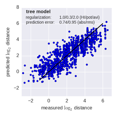
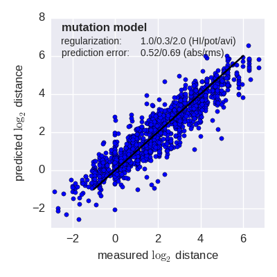
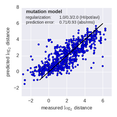
Predicted log2 HI titer distance vs measured HI titer distance for the tree model (top) and mutation model (bottom) fit to A(H3N2) data from the past 12 years. Validation is done either (left) by excluding 10% of all measurements, or (right) 10% of all viruses from the training data. The model is then used to predict the excluded data. The prediction errors are indicted in the figure. When predicting titers for viruses that were completely absent from the training data (right), prediction errors are larger since no virus avidities could be trained.